|
Generating 3D data
By default, the objects that physica manipulates are vectors, i.e. inherently
one-dimensional things. However, one can create a one-dimensional equivalent
of a two-dimensional object by ``unraveling'' the m x n
matrix like this:
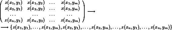
The last line can then be thought of as a mapping
 , where , where

This presupposes that we know
 on a regular array of data points on a regular array of data points

Here's one quick way of creating such a mapping:
generate j 0,,99 100
x=int(j/10)*10
y=j-x
z=(x-50)**2*exp(-0.1*(y-5)**2)
list x,y,z
density\boxes x,y,z
We generated three vectors of length 100, and then interpreted them as a
three-dimensional object. The \boxes switch shows off one more way of
rendering such a ``surface''.
To do the surface justice, however, it is best to perform the reverse: take a
set of vector (1D) data and then create a regularly-spaced grid matrix out of it:
grid x y z m
surface m 25 -30
Note that we have used our regular arrays x, y, and
z to generate a matrix m, but in general grid command
will interpolate data as needed, so the input data representing a
surface
need not be known at a regularly-spaced grid of points
.
For our arrays we could have used the option
grid\nointerpolate since the data is already regularly spaced.
Up: Surfaces, contours, and other 3D plots
Next: Real programming: if's and do's
Previous: Surfaces, contours, and other 3D plots
|